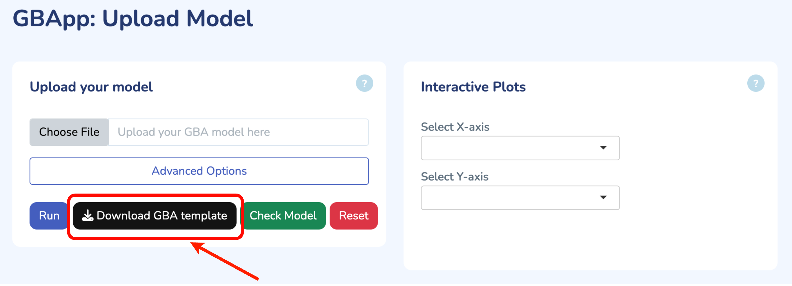
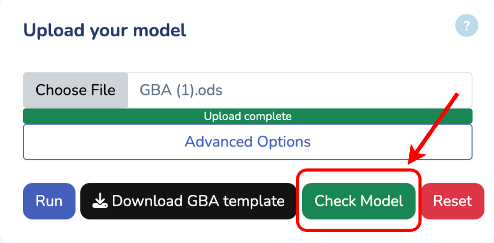
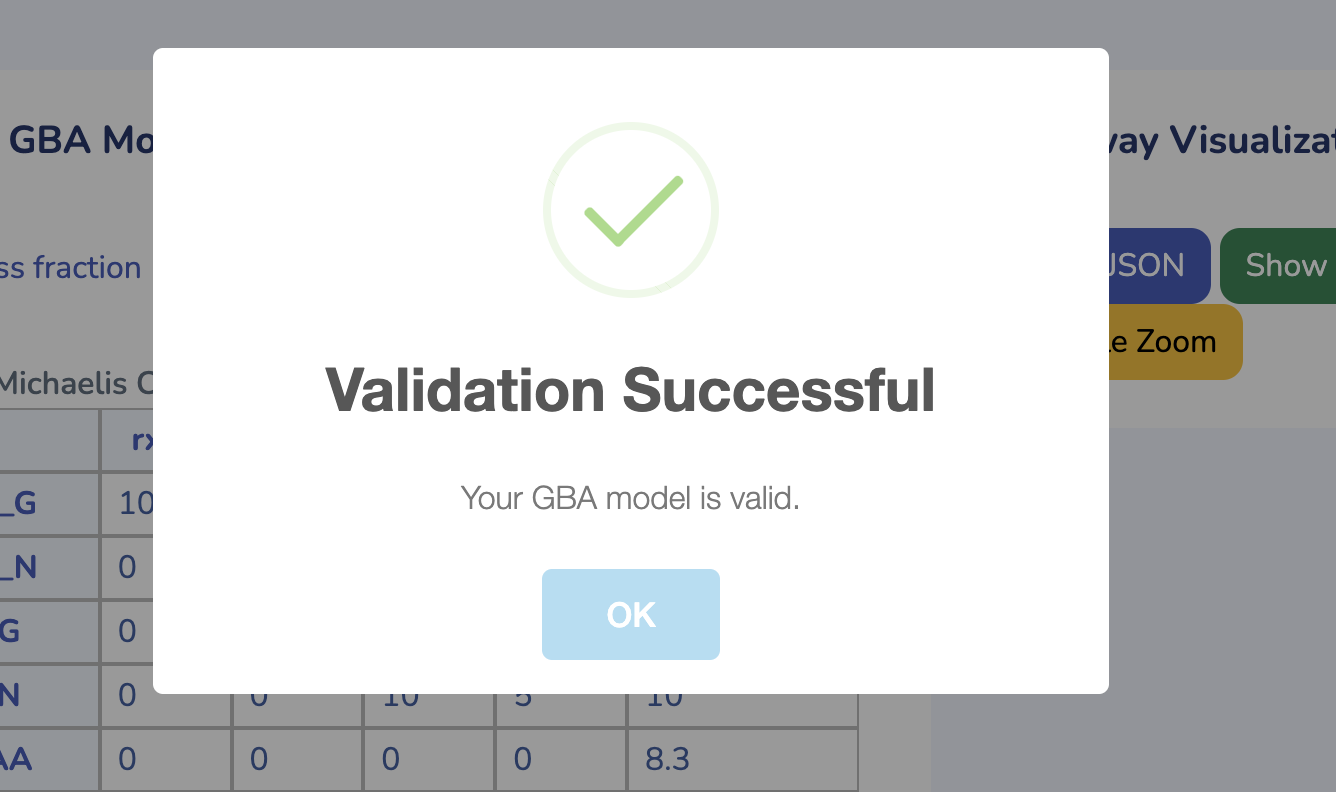
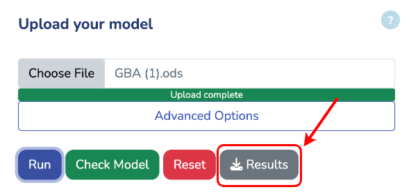
To get started, upload your GBA model by clicking "Choose File" and selecting your .ods file. If you don't have the GBA template yet, you can download it by clicking "Download GBA Template." After uploading your model, ensure its validity by clicking "Check Model." You'll be notified immediately if any issues are detected. For more control, you can use the advanced options to change the solver type for Non-linear Optimization (default is L-BFGS). Once you're ready, click "Run" to begin the optimization process for your uploaded model.
Upload your model

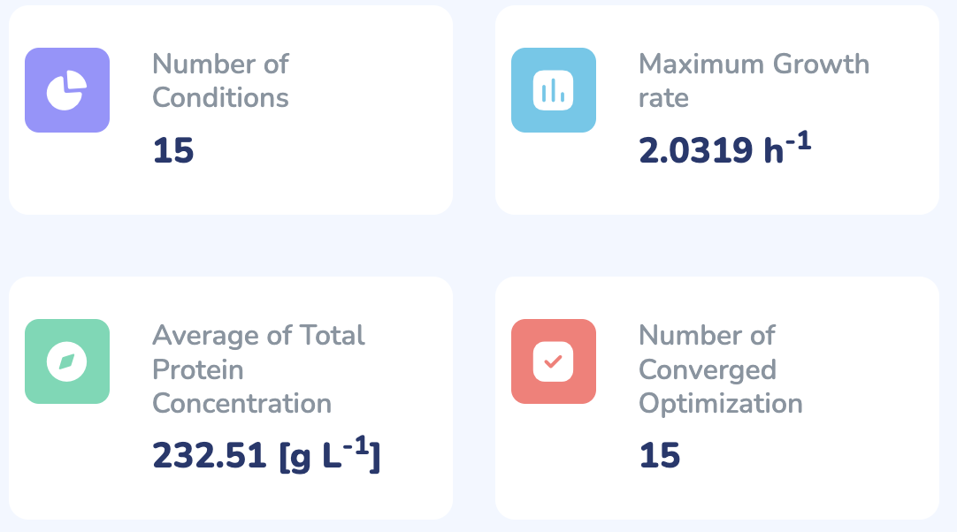
Number of Conditions
Maximum Growth rate
h-1
Average of Total Protein Concentration
[g L-1]
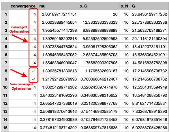
Number of Converged Optimizations
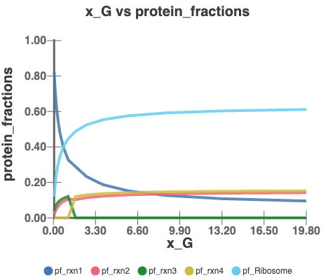
Interactive Plots
In this section, you can visualize the results by selecting different axes, such as Growth Rate, Protein Fractions/Concentrations, Fluxes, and more.
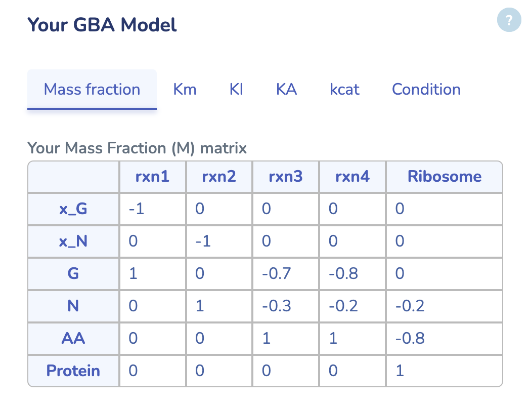
Your GBA Model
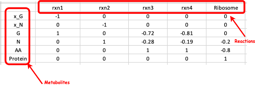
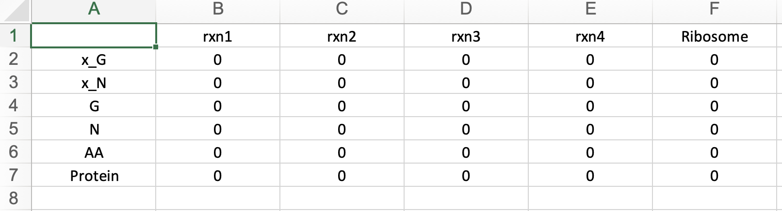
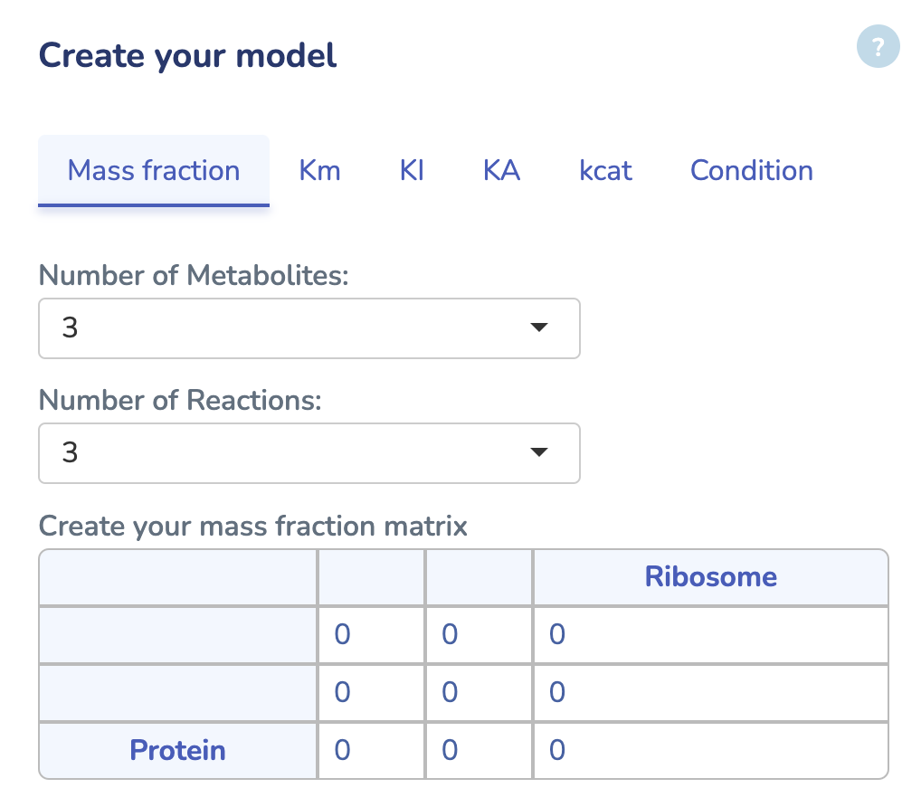
Here, you can view your uploaded GBA model. The first tab displays the Mass Fraction matrix (M) of your model. Even after optimization, you can modify any parameters and rerun the optimization by clicking "Run" in the last tab to see the changes. Additionally, you can download the updated model by clicking "Download" in the same tab.
Here, you can view your uploaded GBA model. The first tab displays the Mass Fraction matrix (M) of your model. Even after optimization, you can modify any parameters and rerun the optimization by clicking "Run" in the "Condition" tab to see the changes. Additionally, you can download the updated model by clicking "Download" in the same tab.
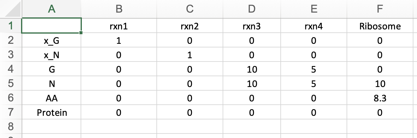
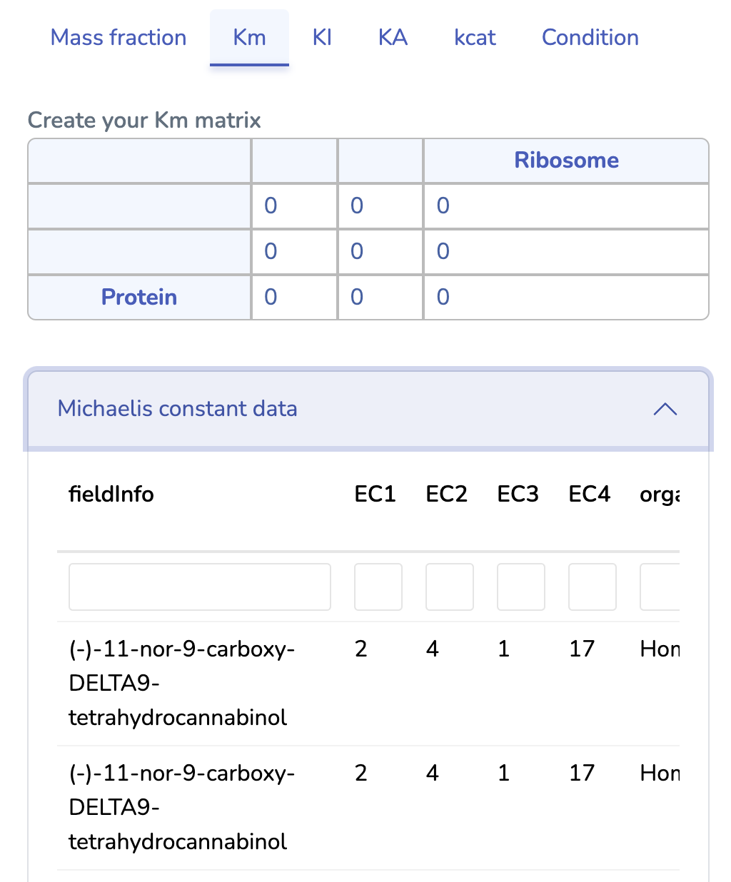
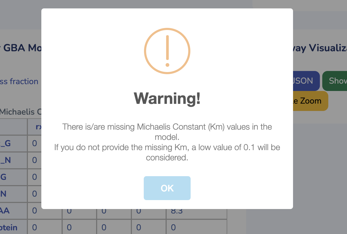
This section displays the Michaelis Constant (Km) matrix of your uploaded GBA model. Make sure each substrate in your reactions has a valid Km value; otherwise, a default value of 0.1 g/L will be used. You can also search for Km values in the table below, sourced from the BRENDA database. Please ensure Km values are mass balanced and converted to g/L by multiplying the Km values in molar units by the molecular weights of the respective substrates.
This section displays the Inhibition Constant (KI) matrix of your uploaded GBA model. You can modify the values directly here.
This section displays the Activation constant (KA) matrix of your uploaded GBA model. You can modify the values directly here.
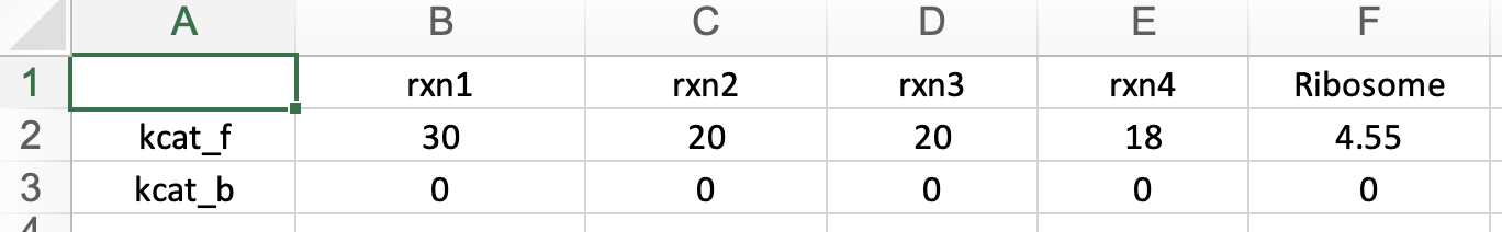
This section displays the Turnover Number (kcat) matrix of your uploaded GBA model. You can search for kcat values in the table below, sourced from the BRENDA database. Ensure that kcat values are mass balanced and converted to 1/h (mass of product/mass of enzyme/hour) by multiplying the kcat values in 1/h units by the molecular weight of the respective product and dividing by the mass of its enzyme. "kcatf" and "kcatb" indicates the kcat for forward and backward reactions, respectively.
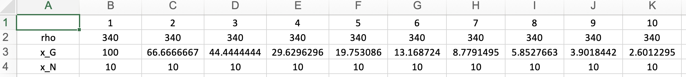
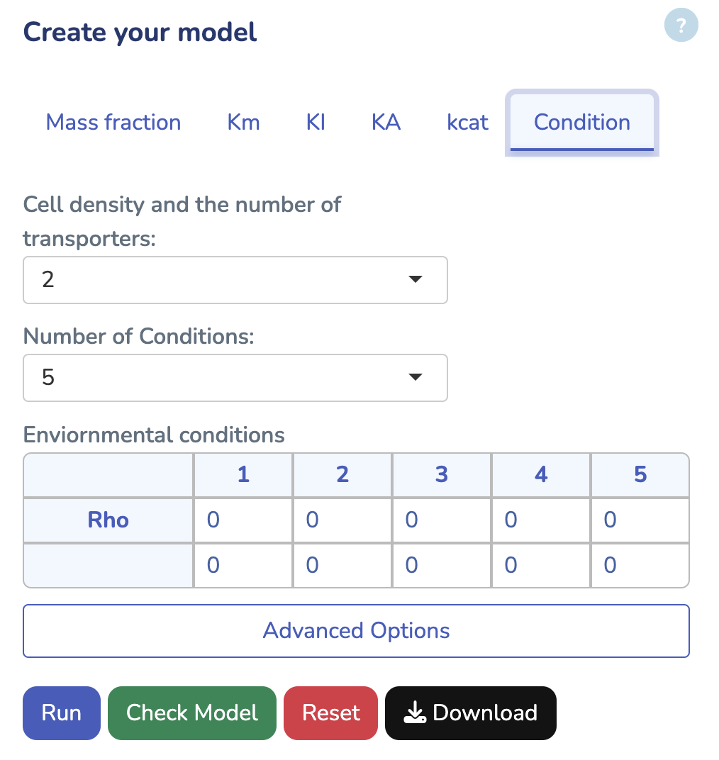
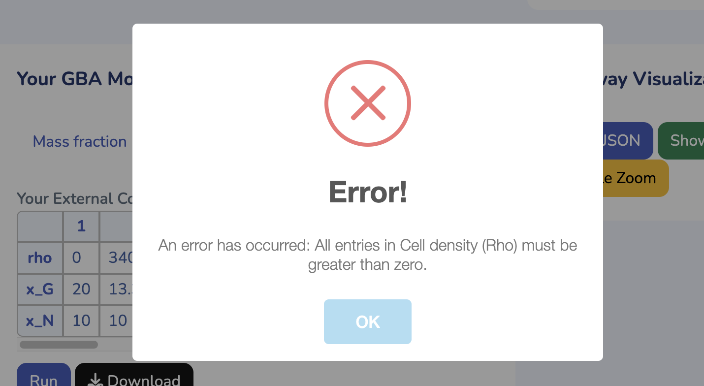
This section displays the External Concentration and Cell Density matrix. The parameter "Rho" represents the cell density in your model, while the other rows show the external concentrations. Ensure that all external concentrations are labeled with "x_". You can modify these values and rerun the optimization by clicking "Run" to see the changes. To download the latest version of your edited GBA model, click "Download."
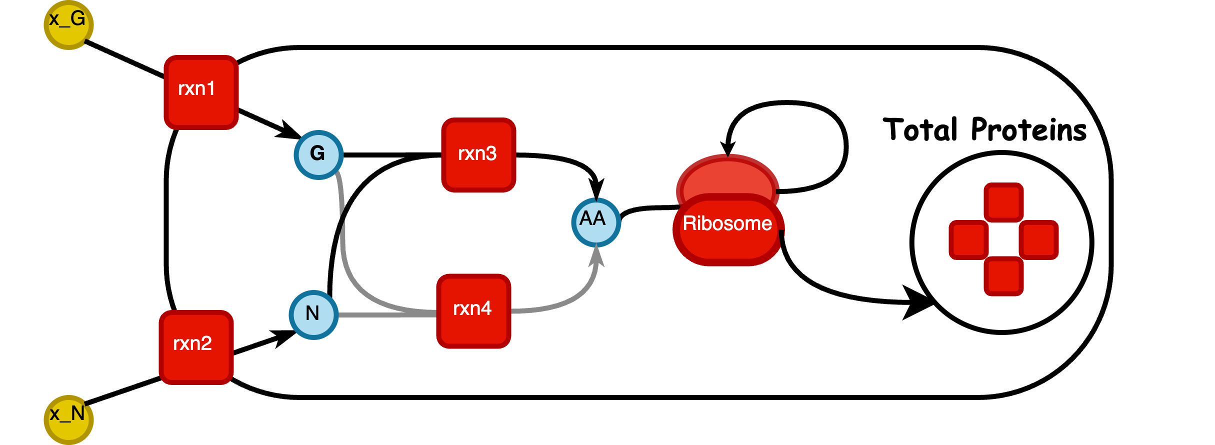
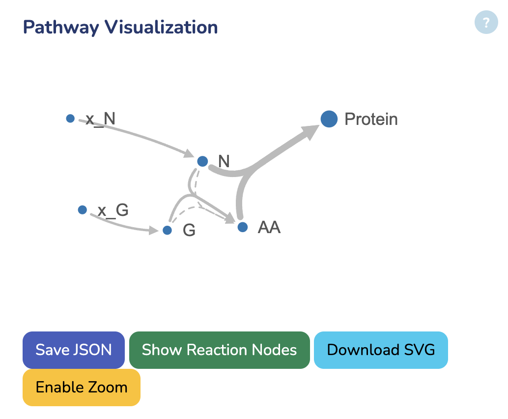
Pathway Visualization
In this section, you can view the network visualization of your GBA model. The dot size represents metabolite concentrations, while the line thickness indicates protein concentrations, both as results from the optimization. You can download the visualization results below.